
Hello everyone,
In this post, I will show you what is CausalImpact, when it is useful and how we can use it in python using the pycausalimpact library.
What is CausalImpact?
In business, you often have to make many decisions and understand the consequences of those decisions. You want to know if your decision improved things or not, and if it was a good one. Basically, you have lots of decisions to make and you want to analyze them to see if they were effective.
In an ideal situation, when making a decision, you conduct an experiment. For example, if you’re deciding on the design of a webpage with many users, you’d set up an experiment. You’d split the users into two groups for example, A and B, and show variant A to one group and variant B to the other. Then, based on the data and results, you’d see which variant performs better. You might use something like a t-test to check for significant differences between the groups. If there’s a significant difference, you know which variant is better and can implement it for all users.
But sometimes, this experimental setup isn’t possible. For instance, if you’re a government leader deciding whether to exit the euro, you can’t just test it with half the country. It’s all or nothing. Sometimes, it’s not ethical or lawful to conduct such experiments, or there simply isn’t enough time to setup an experiment properly.
In such cases, you make decisions without being able to see what would happen with another choice. There’s no way to go back in time and change decisions or see alternate outcomes. Still, we want insights into our decisions, and that’s where CausalImpact analysis comes in.
CausalImpact is a statistical tool developed at Google for estimating the causal effects of interventions in time series data. It addresses situations where randomized experiments are not feasible or ethical, allowing analysts to understand the impact of actions or interventions. The tool computes the counterfactual scenario, which represents what would have happened without the intervention, and compares it with observed data to estimate causal effects. It utilizes a potential outcomes framework, where each unit has potential outcomes under treatment and no treatment. It considers factors such as trends, seasonality, and external variables to ensure robust analysis of time series data. Analysts can use related time series as predictors to improve counterfactual estimation accuracy.
The tool is originally written in R language. But the algorithm is also ported to python and can be used by analysts who are more familiar with python.
how to use CausalImpact in python using pycausalimpact library
As said before, CausalImpact originally developed in R. But, fortunately there is a python library available in python that has the same functionality. in this part I will show you how to install and use it
Install PyCausalImpact
update: “Since pycausalimpact library hasn’t been updated for a while, and I faced difficulties using it with newest version of python, we use another python library called causalimpactx.”
If you are using pip, you can easily install this library using the following command:
pip install causalimpactxIf you are using Conda, you should still be able to install pip within Conda and then use the above command to install causalimpactx library within Conda.
you can install pip within Conda using the command:
conda install pipLoading Data
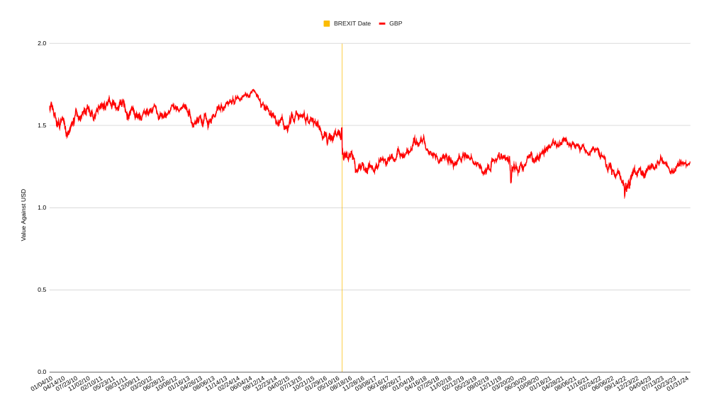
In order to see the causalimpactx python library in action, I selected the effect of BREXIT on GBP value. This is an example for a decision that can not be run as an experiment. Yet we want to have an estimation on what was the effect of exiting the Euro economic zone on the GBP. Before going further, I should say that this is solely for the purpose of working with the library and it can not be considered as a true conclusion by any means. In real world, you can not make such simplifications for a complicated topic like this and you need more through analyses to get a conclusion.
So in this example, we know what happened to GBP value after making the BREXIT decision (Y0). You can see it in the chart below:
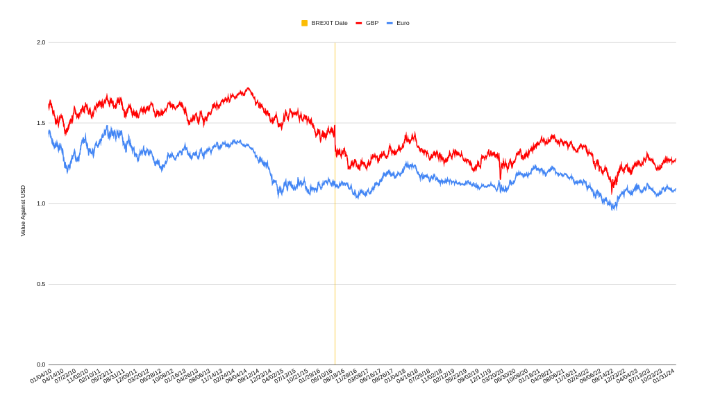
But we don’t know how what could happen if the BREXIT didn’t happen. In order to get an estimation for that, we need to find another time series that had the similar behavior in the per-BREXIT data. We can use the Euro as control for this purpose. See the chart below:
Now we will load this data to causalimpactx library to calculate the counterfactual value. This is the estimation of what could happen if the BREXIT didn’t happen.
First download this CSV that has the above chart’s data:
Next we will load causalimpactx and use pandas library to load this CSV:
import causalimpactx as CausalImpact
import pandas as pd
df = pd.read_csv("Euro - GBP Value- (MetricForward.com).csv")
Analyze Data
We need to set the pre/post intervention periods. It can be done using the following commands:
pre_period = [1, 1691]
post_period = [1692, 3700]
Next, do the calculation:
impact = CausalImpact(df, pre_period, post_period)
impact.run()
Last step is to plot the results:
impact.plot()It gives you three charts similar to the picture below:
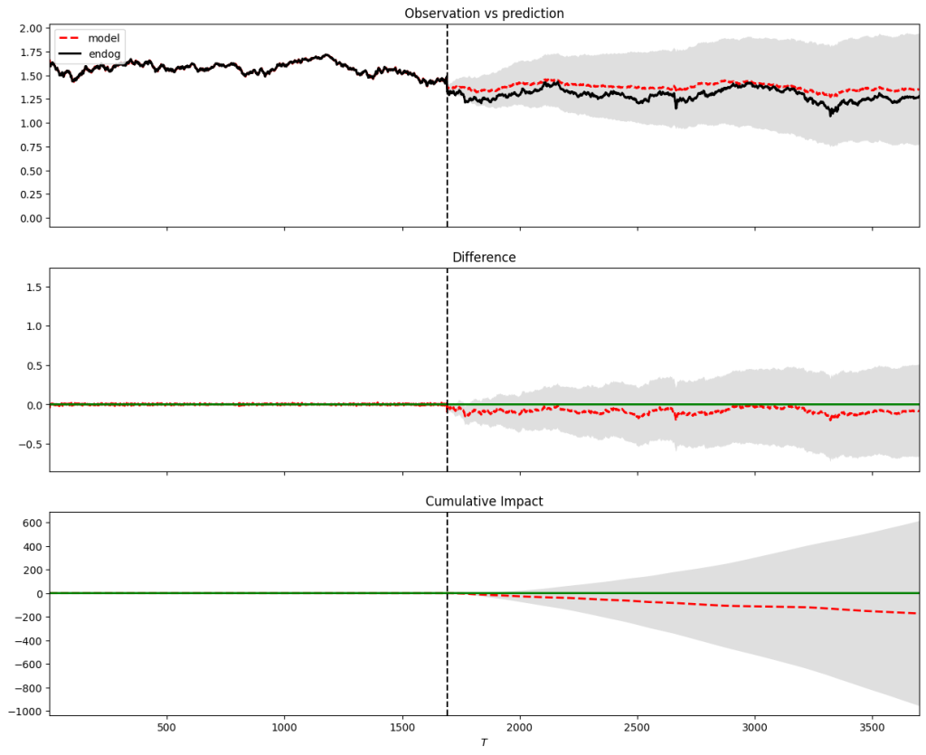
The first chart shows the real values of the time series and what we’d expect without any intervention.
The second chart displays the gap between the real values and what the algorithm predicted.
The third chart illustrates the cumulative difference between the real values and the predicted ones if there was no intervention.
We can also see the summary of calculations as a text using the following command:
impact.summary()It gives you the following output:
                                Average          Cumulative
Actual                             1.29             2591.98
Predicted                          1.38             2764.39
95% CI                     [0.99, 1.77]  [1980.95, 3547.84]

Absolute Effect                   -0.09             -172.42
95% CI                    [0.30, -0.48]   [611.03, -955.86]

Relative Effect                   -6.2%               -6.2%
95% CI                  [22.1%, -34.6%]     [22.1%, -34.6%]

P-value                            0.0%
Prob. of Causal Effect           100.0%
You can also create a basic report by setting the output parameter of the summary to “report”:
impact.summary(output="report")output:
During the post-intervention period, the response             variable had an average value of             approx. 1.29.
By contrast, in  the absence of an intervention, we would have expected an average response of 1.38. The 95% interval of
this counterfactual prediction is [0.99, 1.77]. Subtracting this prediction from the observed response yields an
estimate of the causal effect the intervention had on the response variable. This effect is -0.09 with a 95% interval of
[0.30, -0.48]. For a discussion of the significance of this effect, see below.


 Summing up the individual data points during the post-intervention period (which can only sometimes be meaningfully
interpreted), the response variable had an overall value of 2591.98.  By contrast, had  the intervention not taken
place, we would have expected a sum of 2764.39. The 95% interval of this prediction is [1980.95, 3547.84]


 The above results are given in terms of absolute numbers. In relative terms, the response variable showed  a decrease
of  -6.2%. The 95% interval of this percentage is [22.1%, -34.6%]


 This  means that the negative effect observed during the intervention period is statistically significant. If the
experimenter had expected a positive effect, it is recommended to double-check whether anomalies in the control
variables may have caused an overly optimistic expectation of what should have happened in the response variable in the
absence of the intervention.


The probability of obtaining this effect by                 chance is very small (Bayesian one-sided tail-area
probability 0.0). This means the                 causal effect can be considered statistically
significant.
CausalImpact pitfalls
there are two main things to consider when using CausalImpact:
- The quality of the results really depends on the time series you choose to run the model and calculate the counterfactual value. So, it’s important to select a time series that has a high correlation with the time series you are analyzing.
- You need to ensure that the control time series is not affected by any other factors. In other words, the control time series should remain stable during the post-intervention period. Otherwise, it can easily disrupt your calculations and yield unreliable results.
Final words
In this post I tried to quickly show you how you can do the CausalImpact analysis in python. Please let me know in the comments section if you had any questions or if you had difficulties using the python library.
Additional resources
Original presentation by Kay Brodersen (one of the causal impact creators)
https://arisc.medium.com/how-to-use-googles-causalimpact-ddaa2e770afd