If you are one the excel professionals who has switched to Google sheets from Microsoft excel because your company uses that or for any other reasons, you might miss some of the great features that you had in Microsoft Excel which are not available in Google Sheets. well, you are not alone. I was in the similar situation when I switched to google sheets. One of the features that I missed was the great conditional formatting features in Microsoft excel. For example, the ability to use icon sets for conditional formatting:
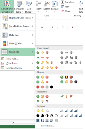
Using this feature, for example, you can set traffic lights based on cell value or you can show a red flag for values that are below the specified threshold. Unfortunately this feature is not available in Google Sheets out of the box. But I will tell you have you can achieve this with a small trick.
It involves 3 steps:
- Create your desired icon set images an uploaded them somewhere that can be publicly accessible over the internet
- Use IF function to define your condition
- Use IMAGE to show the desired icon inside the cell according to the condition
Look at this formula for example:
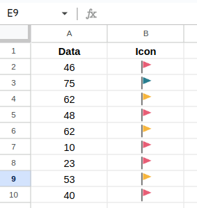
=IF(A2>70,IMAGE("https://metricforward.com/wp-content/uploads/2024/03/GREEN.png"),IF(A2>50, IMAGE("https://metricforward.com/wp-content/uploads/2024/03/YELLOW.png"),IMAGE("https://metricforward.com/wp-content/uploads/2024/03/RED.png"))Here is the result if I write it in cell B2 and copy it down to cell B10:
Now lets take a closer look to see how we achieved this
Explanation
Step 1: How to show the icon inside the cell
In google sheet you can use IMAGE function to show an image within a cell. Here is the syntax for the image function:
= image(URL,mode,height,width)Here is the explanation of every parameter:
- URL: This is the URL for the image. It should be publicly accessible on the internet
- mode (optional): This parameter is an optional indicates how you want to show image in the cell. You can choose a number between 1 to 4:
- 1: Resizes the image to fit inside the cell, maintaining aspect ratio.
- 2: Stretches or compresses the image to fit inside the cell, ignoring aspect ratio.
- 3: Leaves the image at original size, which may cause cropping.
- 4: Allows the specification of a custom size.
- Note that no mode causes the cell to be resized to fit the image.
- Height (optional): This is also optional and indicates the height of image within the cell in pixels. This parameter only needed when you set the mode to 4 (custom size)
- Weight (optional): This is also optional and indicates the wight of image within the cell in pixels this parameter only needed when you set the mode to 4 (custom size)
We can use this function to show an icon inside the cell. For example, if we want to show a red flag within a cell with the size of 24×24, we just need a picture of a red flag uploaded somewhere in the internet that is publicly accessible. Then we just need to pass the URL of that image as a parameter to the image function and set the desired size. I already created and uploaded the picture so you can just use it:
= IMAGE("https://metricforward.com/wp-content/uploads/2024/03/GREEN.png", 4, 24, 24)If you needed publicly accessible icon set images, I created a set of images suitable for icon sets conditional formatting and uploaded them so you can use them out of the box. You can find them in a table at the end of this post.
Step 2: Mix IMAGE and IF functions
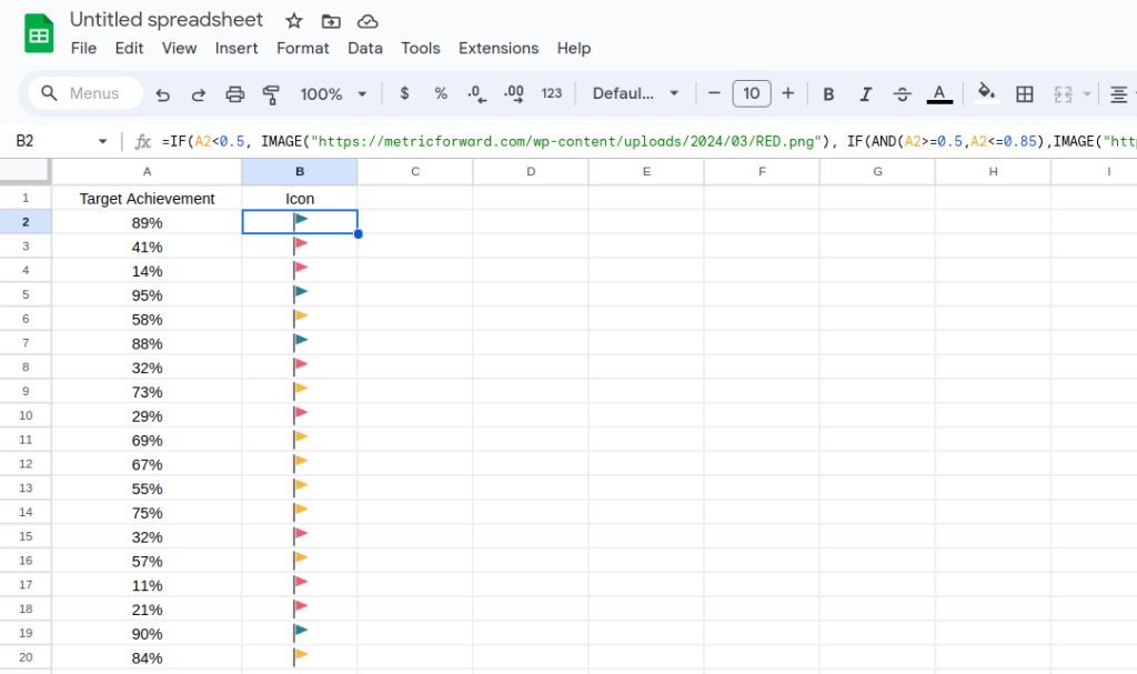
Now that we managed to draw an image within a cell, the only remaining thing is to define a condition using IF function. Lets imagine that you have a sheet for sales targets and in the column A you have target achievement values that can be from 0% to 100%. We want to show a flag based on these criteria:
- IF target achievement is less than 50%, then show a red flag
- IF target achievement is between 50% and 85%, then show a yellow flag
- IF target achievement is higher than 85%, then show a green flag
The IF function equivalent of above sentences is this:
=IF(A2<0.5, show_red_flag, IF(AND(A2>=0.5,A2<=0.85),show_yellow_flag,show_green_flag))We already learned how to show a flag in a cell so lets replace them inside the above function:
=IF(A2<0.5, IMAGE("https://metricforward.com/wp-content/uploads/2024/03/RED.png"), IF(AND(A2>=0.5,A2<=0.85),IMAGE("https://metricforward.com/wp-content/uploads/2024/03/YELLOW.png"),IMAGE("https://metricforward.com/wp-content/uploads/2024/03/GREEN.png")))You might see the below warning. Click allow access to let google load image from the web URL you provided inside the cell:

The result will be the below picture:
Ready to use Icon sets
Depending on the use case, you might need different type of icon sets. I Prepare a group of icon sets that you can easily use in your files. Just right click on your desired icon in the table below and select “Copy image link”.
| Icon set | Icon 1 | Icon 2 | Icon 3 | Icon 4 | Icon 5 |
| Three color Flags |  |  |  | ||
| 5 Stars |  |  |  | ||
| WiFi Antenna |  |  | |  |  |
| Up and Down |  |  |  | ||
| Traffic Lights |  |  |  | ||
| Check Mark / X |  |
I hope this post was useful for you. Please ask any questions in the comments. I will answer them as soon as possible.
سلام یاسین جان
مثل همیشه عالی هستی
پیروز و سربلند باشی
سلام بر شما. سلامت باشید